Advent of Code 2023 or: Things I don’t like about Julia

What began as a quick recap of my experience doing Advent of Code 2023 (my solutions) quickly devolved into a screed about what I dislike about Julia. But first, some math.

Puzzles

This year had lots of stuff for the mathematicians: differentiation and integration (day 9), Jordan curves (day 10), and plenty of linear algebra (day 24, e.g.).

Day 9 - Golf

I’m not much of a golfer, but I couldn’t resist trying my hand on Day 9. The problem is to take an array of integers and find the differences between consecutive terms. We then recursively find these differences until all terms are zero, then use these to “extrapolate” the next value of the sequence by recursively adding (or, in part 2, subtracting). That is, on input 0 3 6 9 12 15, we write

0   3   6   9  12  15   B
  3   3   3   3   3   A
    0   0   0   0   0

then compute A = 3 + 0, B = 15 + A = 15 + 3 + 0. In other words, discrete integration. Here’s the golfed Julia code.

dtz(rows) = iszero(rows[end]) ? rows : dtz([rows; [diff(rows[end])]])
p(i) = sum(sum(d[end] for d in dtz([x])) for x in i)
i = readlines("day9/input.txt") .|> x -> parse.(Int,split(x))
println("Part 1: ", p(i), "\nPart 2: ", p(reverse.(i)))

We are helped tremendously by Julia’s built in diff function that computes consecutive differences.

Day 24 - Linear Algebra

Day 24 was a couple of linear algebra problems in disguise. Solving systems of linear equations is very easy in Julia with its A\b syntax, which is shorthand for solve the system of linear equations given by $A\mathbf{x} = \mathbf{b}$ (suitably encoded).

For Day 24, we were given a collection of “hail stones” with initial position $(x,y,z)$ and velocity $(v_x, v_y, v_z)$. Part 1 simply asked us to determine how many pairs of hailstones meet in a particular square defined by $x$ and $y$ coordinates. With each piece of hail encoded as a pair of tuples ((x, y, z), (vx, vy, vz)), Part 1 boiled down to solving a matrix equation:

function intersection_pt(a, b)
    xa, ya = a[1]
    xb, yb = b[1]
    ma = a[2][2]/a[2][1]
    mb = b[2][2]/b[2][1]
    ma == mb && return [0, 0] # This is outside the square, so idc
    A = [-ma 1; -mb 1]
    c = [ya - ma*xa, yb - mb*xb]
    return A\c
end

Day 24 - Algebraic Geometry

The second part of Day 24 has a nice geometric interpretation. We are given 300 lines in $\mathbb{R}^3$ and asked to find a line meeting all 300 of them. Moreover, each line is parameterized by $\mathbf{p}_i + t \mathbf{v}_i$, and we are told that our line must interesect each line at the right time. That is, if our new line is given by $\mathbf{p} + t\mathbf{v}$, then there is some function $t(i)$ such that $\mathbf{p} + t(i)\mathbf{v} = \mathbf{p}_i + t(i) \mathbf{v}_i$ for all $i$.

Schubert Calculus tells us that there are exactly two lines meeting 4 generic lines in 3 dimensions. In fact, given three skew lines, there is a unique quadric containing them. So to solve this problem we can actually start by computing this quadric for (say) the first three lines, then tracing where each of the remaining lines intersect it. Of course if the lines are chosen at random, then the problem will have no solution, so we assume the problem constructor chose carefully.

Since the line we are trying to construct meets each of the three original lines, it must be in the opposite ruling of the quadric. We identify which line in the opposite ruling by taking the intersection point of some of the remaining 297 input lines with the quadric. By the problem’s construction, these intersection points must be collinear.

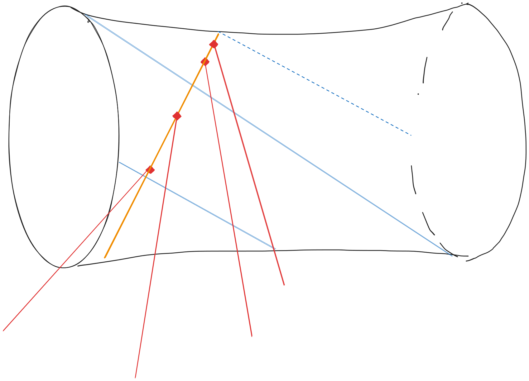
To do this explicitly, we can take three points of each of the first three lines (for a total of nine points) and compute, for each point, the values of each monomial $x^2, y^2, z^2, xy, xz, yz, x, y, z, 1$. The kernel of the 9x10 matrix gives us the quadric. For example, using my input,

using LinearAlgebra
row(p) = [p[1]^2 p[2]^2 p[3]^2 p[1]*p[2] p[1]*p[3] p[2]*p[3] p[1] p[2] p[3] 1]
p = (275325627102914, 177556324137106, 27975811439413)
v = (249, 405, -531)
q = p .+ v
r = q .+ v
p2 = (284428334220238, 231958436807561, 189800593445547)
v2 = (237, 140, -111)
q2 = p2 .+ v2
r2 = q2 .+ v2
p3 = (208260774362545, 354915461185166, 308973039318009)
v3 = (128, -159, -65)
q3 = p3 .+ v3
r3 = q3 .+ v3
M = [row(p); row(q); row(r); row(p2); row(q2); row(r2); row(p3); row(q3); row(r3)]
nullspace(M)

Unfortunately, the built-in linear algebra tools for Julia don’t handle integers very well. Nullspace is computed using the SVD of the matrix and the above actually gives a 10x4 matrix of floats. You can get it to (correctly) remove three of the solutions by specifying the tolerance via the keywords rtol and atol, but the answer you get isn’t precise enough to make this method work.

What you’d like to do is actually cast M as a matrix of rational numbers, which you can force, for example, by making one of the points rational:

p = (Rational{BigInt}(275325627102914), Rational{BigInt}(177556324137106), Rational{BigInt}(27975811439413))

Unfortunately, Julia now breaks when you call nullspace.

julia> nullspace(M)
ERROR: MethodError: no method matching svd!(::Matrix{BigFloat}; full::Bool, alg::LinearAlgebra.DivideAndConquer)

Interestingly, the following linearization of the problem does work, because Julia can solve some (but not all) linear algebra problems with rational numbers. Observe that we have, for each $i$, the equality

where $t(i)$ is the a priori unknown time of intersection. We would like to solve for $\mathbf{p}$ and $\mathbf{v}$. Rearranging, we have

which means $\mathbf{p} - \mathbf{p}_i$ and $\mathbf{v}_i - \mathbf{v}$ are parallel for each $i$. Consequently, their cross-product is zero:

Expanding,

Although this is quadratic, if we repeat this for two values of $i$, say, $i=1$ and $i=2$, then both have the same quadratic term $\mathbf{p} \times \mathbf{v}$ and we can subtract them to get a linear equation. If we repeat this twice, then we get two vector equations or 6 linear equations in 6 variables. We can then solve this:

cross_coeffs(a) = [0 -a[3] a[2]; a[3] 0 -a[1]; -a[2] a[1] 0]
function part2(hail)
    p1, v1 = hail[1][1], hail[1][2]
    p2, v2 = hail[2][1], hail[2][2]
    p3, v3 = hail[3][1], hail[3][2]
    A, B, C, D = cross_coeffs.([p2 .- p1, v2 .- v1, p3 .- p2, v3 .- v2])
    M = Rational{BigInt}.(vcat(hcat(A, B), hcat(C, D)))
    rhs = [cross(p1, v1) - cross(p2, v2); cross(p2, v2) - cross(p3, v3)]
    return M\rhs
end

Unlike nullspace, \ apparently forces Gaussian elimination when called on a Rational{T} matrix and the above gives a precise answer to Part 2.

Julia

My overall impression of Julia is favorable. It’s easy to write, fast (fast fast), and has excellent tooling. Nevertheless, it’s more fun to point out frustrating things than congenial ones, so that’s what the rest of this post is dedicated to. Below is a list of the most annoying things I encountered in Julia.

1. Too many options?
2. Weird points of friction
3. The type system is frustrating
4. Seriously, what’s up with types?

1. Too many options

Julia provides multiple ways to express the exact same thing (even identical AST’s). For example, the following are equivalent:

for i in 1:100
    # do whatever
end

for i = 1:100
    #...
end

for i ∈ 1:100
    #...
end

Or consider what I should do if I have multiple functions I want to chain together. For example, suppose I want to extract the first element of some iterable that is greater than 3. In Python, there’s basically one way to do this:

[i for i in my_iterable if i > 3][0] # easy
next(i for i in my_iterable if i > 3) # preferred

Julia has many more, and they can be pretty different. Here’s just a few:

[i for i in my_iterable if i > 3][1] # matches python
first(my_iterable |> filter(>(3))) # preferred?
my_iterable |> filter(>(3)) |> first # is this different?
(first ∘ filter(>(3)))(my_iterable) # ?

Note that we can replace the argument >(3) in filter with an anonymous function t -> t > 3 too if we want.

Adding some complexity here is the fact that the filter function behaves very differently from a typical Julia function. The usual syntax is filter(f, a), where f returns a bool. However, if you call filter(f), then Julia creates a partial function, making filter more available for piping. This is hard-coded behavior of the filter function. It doesn’t work in general. For example,

function my_func(f, a)
    return sum(f.(a))
end

my_func(x -> 2*x, [1,2,3]) # returns 12
[1,2,3] |> my_func(x -> 2*x) # MethodError

Furthermore, the pipe operator has a very unexpected precedence:

julia> 1:5 .> 3 |> sum
5-element BitVector:
 0
 0
 0
 1
 1

 julia> (1:5 .> 3) |> sum
 2

(Note that this does match the operator precedence of |> in R, which is presumably the entire reason for this insanity.)

I’m not the first person to be bothered by this. I ventured on Julia’s comically hostile discourse forum and found a contributor slowly losing his mind as he suggests then rejects a sequence of increasingly convoluted solutions to piping issues: one, two, three.

2. Weird points of friction

Julia made a few surprising design decisions early on that I think were mistakes. Namely: 1-indexing and aggressive unicode support.

1-indexing is a sticking point for a number of programmers. It’s not hard to switch between 1- and 0-indexed languages, but it’s an odd place to completely upend modern conventions. The fact that Julia’s target audience (academics, mostly) may be more familiar with the 1-indexed languages R and MATLAB isn’t really a good enough reason for me.

The unicode support is wild. You can use basically any unicode character in a token if you want. Julia base includes a fair amount of it already. See, for example, the function composition operator ∘ I used above. There’s also an infix xor given by the exotic ⊻. Julia codebases are littered with these characters. In fact, it seems to be somewhat of a point of pride of the Julia community that they are able to create more one-character variable names than any other programming language.

In addition to easily avoidable own-goal design choices, Julia has a few things that are unexpectedly hard to handle. Most prominent among these is optimization. In short: Julia is difficult and often counterintuitive to optimize.

Consider, for example, the following functions. Which is faster?

function f(x::Vector{Int64})
    r = []
    for i in x
        push!(r, i)
    end
    return r
end

function g(x)
    r = Int64[]
    for i in x
        push!(r, i)
    end
    return r
end

It’s g. By a lot.

julia> x = [i for i in 1:10000]
julia> @btime f(x)
141.600 μs (9498 allocations: 474.80 KiB)

julia> @btime g(x)
56.000 μs (9 allocations: 326.55 KiB)

This has to do with the arcane processes of type inference in Julia, which brings me to

3. The type system is frustrating

What’s going on in the above example? The first unintuitive fact is that putting the type of x in the function signature provides the compiler with no useful information to use in optimization. The JIT will not compile a method until it’s called, so even though g is defined on any type, we never created a method defined on anything other than a vector of Int64’s.

In particular, all the type inference available to Julia when compiling f is also available to it when compiling g. So there’s no improvement from declaring the type of x. On the other hand, the type of r does not get inferred even though it’s possible to do so. Why not? Because r = [] actually means r = Any[]. So we’ve implicitly declared the type of r in the function f even though we didn’t mean to.

That’s why g is faster. It has a correctly typed vector, so the memory allocation is far more efficient. Consider now

function h(x::Vector{T}) where T
    r = T[]
    for i in x
        push!(r, i)
    end
    return r
end

This is the same as g (they are, in fact, identical functions).

julia> @btime h(x)
56.100 μs (9 allocations: 326.55 KiB)

So that’s surprising. I learned about this type of optimization after Advent of Code and reduced my solve times on several puzzles by more than 60%.

Consider another example suggesting that you should probably never put type annotations in a function signature.

f(x)::Int64 = x
f(2) # returns 2
f(2.0) # returns 2 (!!!!)
f(2.5) # InexactError

g(x) = x::Int64
g(2) # returns 2
g(2.0) # TypeError
g(2.5) # TypeError

This happens because the notation function(args...)::T attempts to cast the return value of f as T. The notation expr = x::T is a type assertion that x has type T. Here’s a more expanded example

function s(x)
    y = x::Int64
    return y
end

function t(x)
    y::Int64 = x
    return y
end

Which of these errors when x=2.0? It’s actually s, not t! I cannot fathom why the language was designed this way.

4. Seriously, what’s up with types?

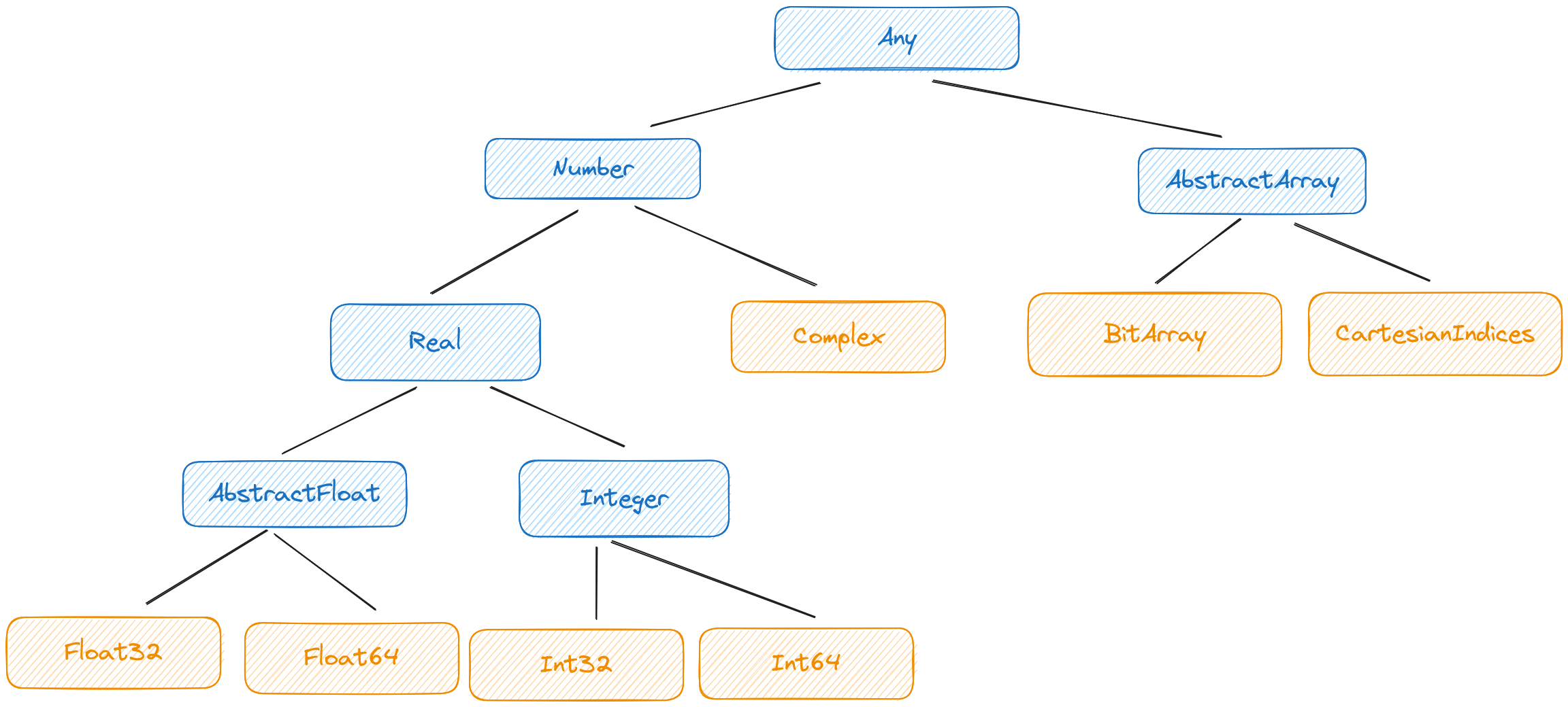
Julia has types. Those types are organized into a type hierarchy that obeys certain rules.

1. The type hierarchy is a tree with root node Any
2. A type may either be abstract or concrete
3. Abstract types cannot be instantiated
4. Concrete types cannot have subtypes

Together, these rules make for a very flexible, safe type system. Since Julia uses dynamic (multiple) dispatch, it’s easy to define methods for entire branches of the type tree. For example,

julia> foo(x::Number) = x+1
foo (generic function with 1 method)

julia> foo(x::String) = x*"asdf"
foo (generic function with 2 methods)

julia> foo(2.0)
3.0

julia> foo("bar")
"barasdf"

This is praxis in Julia world:

[…] definition of function behavior by dispatch is quite common – idiomatic, even – in Julia.

(Julia Docs)

Type hierarchies, and type digraphs more generally, are common in object-oriented languages because they allow subtypes to easily inherit behavior. I can define a method for Number and know that the Julia compiler will automatically try to execute that method for all descendents of Number.

The insight made by Julia is that this process is not related to the process of adding new types to existing behaviors. In OOP, the correct way to add a type to my foo method defined above would be to declare it as a subclass of an existing class in order to inherit behavior from its antecedents. In Julia this is not necessarily correct (it would be, though, if my new type were a subtype of Number).

Indeed rule 4, that concrete types cannot have subtypes, almost completely forbids this. Moreover, if I have a new type that I want to add multiple existing methods to, then rule 3 prevents me from doing this inside the type hierarchy unless those behaviors can all be inherited from a single abstract type. Again, this is designed to eliminate an OOP-style problem—in this case, the “diamond” problem.

Instead, you are meant to add methods to new types by simply declaring them. For example, I can define a new type and add a foo method to it like this:

julia> struct Bar
    a::Int64
    b::Int64
end

julia> foo(x::Bar) = x.a + x.b

There’s a hidden consequence of this approach to typing. If I want to create a fairly generic function, say a mathematical function that should work on numeric types, it is most correct and idiomatic to not specify the argument types in the function definition. This gels with what we saw above: declaring argument types also does not help performance.

Indeed by not stating argument types, I allow for the possibility of other coders defining their own numeric types and running my algorithm on them. Unfortunately, these considerations lead to the central contradiction at the heart of Julia’s type system. The following things are all simultanesouly true:

1. I should not put type arguments in function definitions to allow for greatest flexibility
2. I must put type arguments in function definitions to allow for full use of multiple dispatch
3. I cannot specify any interfaces (read: traits) that function arguments must satisfy without using a type

For this reason, the subject of Rust-like traits has become a popular discussion topic among Julia users (see here for a concrete proposal). Many argue that Julia already has traits via Tim Holy’s “Holy” Trait Trick which exploits Julia’s robust types-as-data philosophy. This, unfortunately, doesn’t really cut it. Solving the 1-3 contradiction above requires a trait system that provides a simple interface for both package authors and consumers. In particular, package authors need to be able to communicate the trait interface within the trait itself; they cannot expect users to read their source code to understand how the trait needs to be implemented.